Mastering VLOOKUP in Google Sheets: Your Ultimate Guide

Do you find yourself swimming in a sea of data, desperately trying to locate that one specific piece of information? If you’re a Google Sheets user, you’re in luck! VLOOKUP in Google Sheets is your trusty lifesaver in the world of spreadsheets. In this guide, we’ll break down the concept of VLOOKUP into bite-sized, easy-to-understand explanations, complete with analogies and examples, so you can confidently use it like a pro.

What is VLOOKUP?

Imagine VLOOKUP in Google Sheets as your personal detective in a massive library, helping you find a specific book. It stands for Vertical Lookup, and it’s designed to search for a value in a vertical column (like a list of books’ titles) and return a related value (like the book’s author) from the same row.

The VLOOKUP function looks like this =VLOOKUP(search_key, range, index, [is_sorted]). Let’s start by breaking this down.

The search_key is the value you want to look up, which in this scenario is your book title. This can either be text in quotes eg “Harry Potter”. Or you can have it refer to a certain cell. As we discussed in our article The Ultimate Google Tutorial For Newbies. This is one of the boxes in the grid where you enter data.

The range is where you are searching for the value (the library’s catalog). The index is the column number from which you want to retrieve data (the author’s name).

Lastly is the optional value is_sorted that needs to be set to TRUE if your data is sorted, or FALSE if it’s not. If this value is not provided then it is assumed the data is sorted. It is generally good practice to enter this value despite being optional.

Let’s Put It into Action

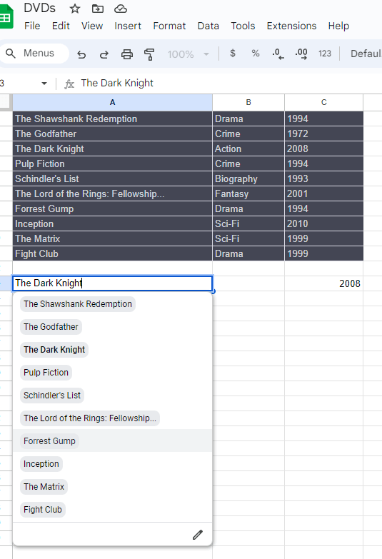
Imagine you have a spreadsheet for your DVD collection, and you want to find the release year of a specific movie.

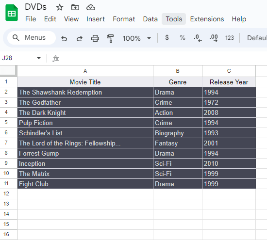
Here’s how you can use VLOOKUP:

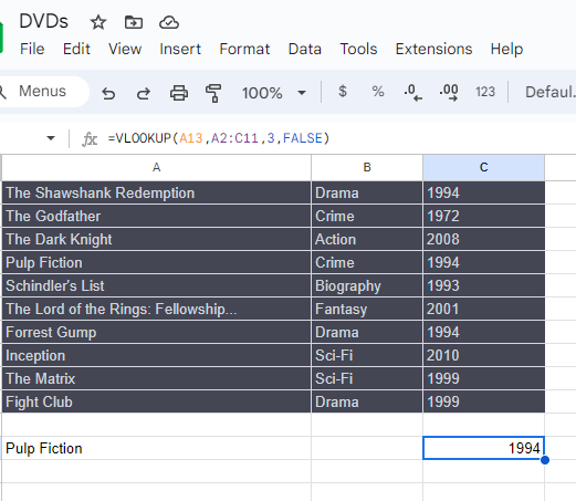
Let’s say you want to be able to enter a Movie name in Cell A13 and have the Release Year appear in C13.

Click on cell C13 and Type =VLOOKUP( into the cell. Click on the field with your search_key which in this case is the title you want to search for which is A13 followed by a comma.

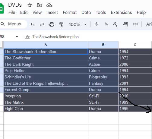
Now you need to define the range you will be searching for the values in. Click on Cell A1 and drag your cursor, you will see the cells highlighting. Make sure to drag the box so it covers all of the data and then type a comma.

Determine which column has the information you want to retrieve. In our case, it’s the column with release years. Count how many columns are to the right of the first column in your selected range (starting from 1). This is your index. For release years, in this case would be 3 followed by another comma.

Specify the sorting which as mentioned above is generally Optional. But in our case, it is required as our list is not sorted, so type FALSE.

Finish the formula by typing ) and pressing Enter.

And voilà! You’ve just used VLOOKUP to find the release year of your movie.

FAQ: Common Mistakes to Avoid

Incorrect Range Selection

Selecting the wrong range is like searching for a book in the wrong library. Double-check that your range includes both the column with the search key (movie titles) and the column with the data you want to retrieve (release years).

Exact Match Required

VLOOKUP defaults to finding an exact match. If you don’t find a match, it returns an error. To avoid this, you can use the is_sorted argument and set it to FALSE. This way, VLOOKUP will find the closest match.

Understanding Relative Cell References

When copying your VLOOKUP formula to other cells, make sure to use relative cell references. Google Sheets will automatically adjust the formula to look in the right place. If you use absolute references (like $A$1), it won’t work correctly when copied. We will be covering this in another article soon.

Conclusion

Mastering VLOOKUP in Google Sheets is like having a GPS for your data. It helps you navigate your spreadsheet with ease, retrieving the information you need precisely and quickly. With the simple steps outlined in this guide, you’ll be well on your way to becoming a spreadsheet maestro.

Remember, practice makes perfect! So, open up Google Sheets and start using VLOOKUP to streamline your data tasks today. You could take it a step further and look at data validation to populate a drop-down list so you can select the relevant title.

Now that you’ve mastered VLOOKUP, you’re ready to tackle your data challenges efficiently and accurately. Happy spreadsheeting!